Identifying Migration Arifacts and Reflectors by Machine Learning Methods
by Yuqing Chen
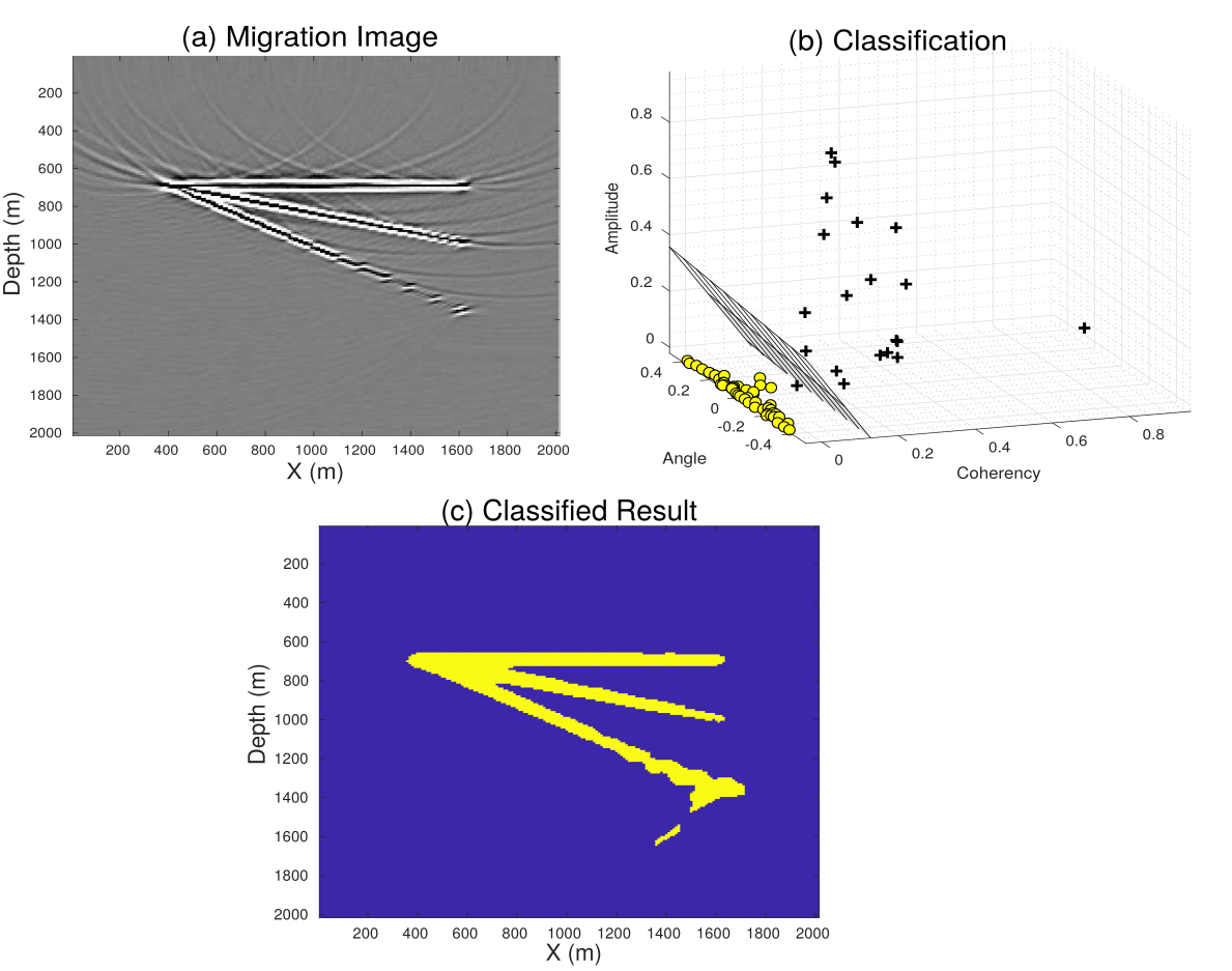
Figure 1 (a) Migration image of a three layer model with some artifacts which caused by sparse geometry, (b) classifiction results of training set and (c) classification results of all imaging points in the migration image.
In this lab, the support vector machine (SVM), neural network (NN), and logistic regression algorithms are used to distinguish artifacts and reflectors point in a migration image.
-
Matlab
- Find features with dimension N. In our case, we choose the coherency, dipping angle and amplitude as our features, so N = 3.
- Build training sets. Manually pick 50 artifact points in the image and labeled as 0, then manually pick 30 reflector points in the image and labeled as 1.
- Use machine learning algorithms to estimate an optimal N-1 dimension boundary which separates the training set. In our case, the boundary is a 2D surface.
-
Input the rest of points in the image into the trained model to do classification.
Download the codes Comparision.zip and unzip it. Change your Matlab working directory under this file so you may able to use all necessary sub-functions. The main function is “compare_main.m”, open it in the Matlab script and click “run”. The comments in the code can help you understand the code.
- The function costFunction2.m and nnCostFunction.m are used to compute the gradient and misfit of the logistic regression and neural network, respectively. For the SVM, the function svmTrain.m is used to train the model parameters. This function is in courtesy of Prof. Andrew Ng from his Machine Learning course from Coursera (https://www.coursera.org/learn/machine-learning/home/week/7).
- Load the migration image and corresponding 3 features: “cohe”, “angl” and “engy” represent the coherency, dipping angle and the amplitude, respectively.
- As different features have the different unit, we rescale them into the range between -1 to 1.
- Manually pick 50 artifact points in the image and labeled as 0, then manually pick 30 reflector points in the image and labeled as 1 to build the training set.
-
Randomly initialize the initial model parameter and then compute the gradient and update the model parameter by Steepest descent method.
The theory of support vector machine (SVM) is different compared to the logistic regression and neural network. SVM separates different class of data with a clear gap that is as wide as possible.
minθ, bd = (1)/(2)θTθ
subject to
y(i)(θTx(i) + b) ≥ 1
where the parameter θ and the interception term b controls a boundary that separates different class of data. This equation can be transformed into a dual problem to solve for the optimal θ and b.- Try to train the model with an unbalanced training set. For examples, we have 50 artifacts points and 3 reflector points in the training set.
- Modify the program as follows: (1) For each image point in the migration image, open a local window with size of winx by winz around this image point. (2) Unroll this local image to the size of 1 by winx*winz and saved as one example in the training set. so in this case, the dimension of input features are winx by winz).
-
Train the model and compare the predicted classes to the actual classes.
Please let me know if there are any errors in this Lab, please contact: yuqing.chen@kaust.edu.sa
Regards,
Yuqing Chen