Two-Point Ray Tracing Lab
by: Abdullah AlTheyab
date: Oct 6, 2012
Objective:
- get familiar with ray tracing
- know different methods for two-point ray tracing
- realize the deficiencies of each method
Procedure:
- Download the lab package from here and unpack the downloaded file and make the unpacked directory the working directory in MATLAB. In MATLAB, open the file main.m
- Follow the instructions in the MATLAB script file
- After finishing the required work, in MATLAB write publish('main.m')
Contents
Building a testing velocity model
This is just one testing model. Feel free to change it. Note that ray tracing works better in smooth models. Use the "mysmooth.m" tool to smooth your velocity model
These parameters has to be set currently. If you use your own velocity model change these parameters accordingly.
h=25; %m sampling interval of the velocity field
N1=100;% number of elements in the z-direction
N2=200;% number of elements in the x-direction

vel=(1:N1)'*((1:N2)*0+1)*20+700;
vel(1:N1/2,:)=vel(1:N1/2,:)+500;
vel(1:N1/5,:)=vel(1:N1/5,:)*0+1500;
vel=mysmooth(vel, 2);
imagesc(h*(1:N2), h*(1:N1), vel); colorbar();
xlabel('x[m]'); ylabel('z[m]');
title('Testing velocity model');

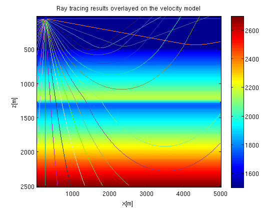
Shooting rays
In this part, we simply shoot rays from a source point without knowing where the ray is heading to.
TODO:
- move the source position deeper.
- currently the take-off range is from 0 to pi. Generate another plot by copying the following code and change the range of take-off angles to contain only one take-off angle the ray reaches the surface at x-position 3000m. Can you find another ray that reaches the same position?!
srcpos=[2;10]; % source point position [z,x] in grid coordinates 1<=srcpos(1)<=N1 & <=srcpos(2)<=N2
imagesc(h*(1:N2), h*(1:N1), vel); colorbar();
hold on;
for ang=0:pi/2^5:pi % the range of take-off angles of the rays from the source point
    p=[sin(ang);cos(ang)]; % ray parameter
    [rayx, rayz, rays, rayt]=tracer(vel, h, h, p, srcpos, 20000); %ray tracing
    plot(h*rayx, h*(rayz),'color',[rand rand rand]); % ploting the ray
end
plot(h*srcpos(2), h*srcpos(1), '*');
hold off;
xlabel('x[m]');
ylabel('z[m]');
title('Ray tracing results overlayed on the velocity model');
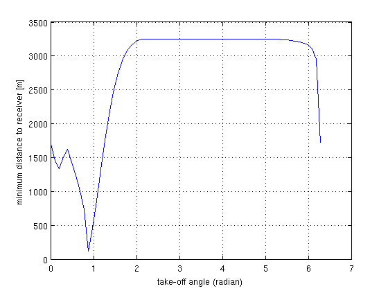
Two point ray-tracing by searching for the optimal take-off angle(s)
The optimal take-off angle will send the ray right to the receiver. This is a non-linear optimization problem because there could be many ray paths between the source and receiver. Why? Before we choose the optimal angle, we search a sample set of all possible angles and find the closest ray to the receiver. What we get is a function of how close the ray came about the receiver. A ray that connect the source to the receiver should have zero distance from the receiver.
TODO
- See the following figure. Does the function touch zero value? Try increasing the sampling of take-off angles search?
- Move receiver position. How does the distances change?
srcpos=[1;10];  % source point position
recx=120;        % receiver x-position
recz=70;        % receiver z-position
% search variables
samp=pi/2^5;     % seach interval
optangl=0;      % optimal take off angle
mindist=10000;
arange=0:samp:2*pi;
dist=arange*0;
for iang=1:length(arange) % the range of take-off angles of the rays from the source point
    ang=arange(iang);
    p=[sin(ang);cos(ang)]; % ray parameter
    [rayx, rayz, rays, rayt]=tracer(vel, h, h, p, srcpos, 20000); %ray tracing
    val=min(sqrt((h*(rayx-recx)).^2+(h*(rayz-recz)).^2));
    dist(iang)=val;
    if(val<=mindist)
        optangl=ang;
        mindist=val;
    end
end
plot(arange, dist);
grid;
xlabel('take-off angle (radian)');
ylabel('minimum distance to receiver [m]');
- Does the ray touches the receiver? how is that related the function above?
p=[sin(optangl);cos(optangl)]; % ray parameter
[rayx, rayz, rays, rayt]=tracer(vel, h, h, p, srcpos, 20000); %ray tracing
imagesc(h*(1:N2), h*(1:N1), vel); colorbar();
hold on;
plot(h*rayx, h*(rayz),'color',[rand rand rand]); % ploting the ray
plot(h*srcpos(2), h*srcpos(1), 'r*');
plot(h*recx, h*recz, 'k*');
hold off;
grid;
xlabel('x[m]');
ylabel('z[m]');
title('Two-point ray tracing results overlayed on the velocity model');
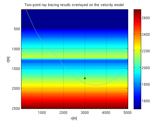
We can do a local-gradient optimization (like steepest decent) to find the ray that actually connect the source to the receiver. The optimal trace found by the search method above could be used as a starting solution of the optimization.
TODO
- How would you search for every possible ray paths between the source and receiver?
- Comment on this exhaustive search method in terms of cost? Consider a big survey that has 100's of shot points and 100's of receivers.
Two-point ray-tracing using Fermat's principle
According to Fermat's principle, the ray-path that connects two points in the medium is the minimum time ( ) path. A ray path can be parametrized a series of points {(xsrc, zsrc), (x1, z1), (x2, z2), ..., (recx, recz)}.
We can solve for the pairs (x1, z1), (x2, z2),... that minimize the traveltime of the ray. This a non-linear problem that involve numerical calculation of derivatives  and
and  .
.
For VSP survey with transmitted waves, the z1, z2,... are fixed at incrementing values, and we solve only for x1, x2, ...etc. This assumes VOZ and no head/diving waves, because that would require at least two z-values to be equal.
% test velocity model
nz=50; nx=50;
vel=ones(nz,nx)*2000; % unit: m/s
vel( 5:10, :)=1500;
vel( 20:25, :)=3000;
sln=1./vel;
h=10; % grid spacing unit:  m
imagesc((1:nx)+.5, (1:nz)+.5,  vel); colorbar; grid on;
% geometry
r_x=1;
s_z=1;
ns=10:10:nx;%2:2:nx;
nr=40;%2:2:nz;

[rays_z, rays_x]=getRays(sln, nz, nx, ns, nr, s_z, r_x, h);
raysz_orig=rays_z;
raysx_orig=rays_x;

% Plotting the rays
imagesc(h*((1:nx)+.5), h*((1:nz)+.5),  vel); colorbar; grid on;
hold on;
for is_x=1:length(ns)
    s_x=ns(is_x);
    for ir_z=1:length(nr)
        r_z=nr(ir_z);
        nseg=length(s_z:sign(r_z-s_z):r_z);
        ray_z=reshape(rays_z(is_x, ir_z, 1:nseg), 1, nseg);
        ray_x=reshape(rays_x(is_x, ir_z, 1:nseg), 1, nseg);
        plot(h*ray_x, h*ray_z, 'color', [rand rand rand]);
    end
end
hold off;
xlabel('x[m]');
ylabel('z[m]');
title('Two-point ray tracing using Fermat''s principal');
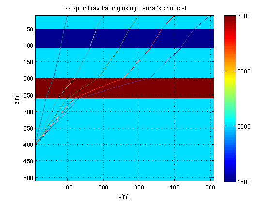
The method above will give the nearest Fermat ray to the starting solution. This way we can choose which ray we want by having a starting ray close to it. Nevertheless, this is not the most efficient method if we want the raypaths of first arrivals.
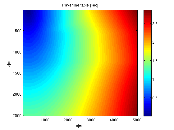
Two-point ray-tracing using traveltime tables
Traveltime are fast to compute. So they can be used in ray tracing. The first arrival ray path is the steepest descent path from the receiver to the source in the traveltime table. So, we can get the ray path by applying the steepest decent method with fixed step length.
TODO
- Move receiver to z=5. What ray is found now?
- Local gradient methods like steepest decent assume continuous differentiable functions. Are traveltime tables differentiable everywhere? Where would the traveltime table be discontinuous? Can you break this method based on this weakness?
% test velocity
n1=100;
n2=200;
h=25;
vel=(1:n1)'*((1:n2)*0+1)*10+1200;
vel(1:n1/2,:)=vel(1:n1/2,:)+500;
vel(1:n1/5,:)=vel(1:n1/5,:)*0+1500;
vel=mysmooth(vel, 1);
sln=1./vel;

% calculating traveltime table
srcx1=2; % source position
srcx2=10;% receiver position
ttbl=mysmooth(tt(sln, n1, n2, h, srcx1, srcx2),2);
imagesc(h*((1:n2)), h*((1:n1)), ttbl); colorbar;
xlabel('x[m]');
ylabel('z[m]');
title('Traveltime table [sec]');
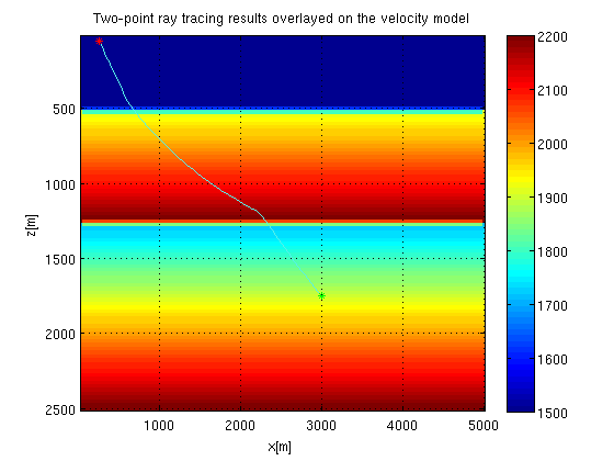
raypath by steepest decent
recx1=70; % receiver z-position
recx2=120;% receiver x-position
dtdz=diff(ttbl, 1, 1);
dtdz=[dtdz; dtdz(n1-1,:)];
dtdx=diff(ttbl, 1, 2);
dtdx=[dtdx dtdx(:,n2-1)];
x=[recx1; recx2];
nitr=500;
path=zeros(nitr, 2);
for itr=1:nitr-1
    path(itr, :)=x;
    ix1=int32(x(1));
    ix2=int32(x(2));
    if(abs(ix1-srcx1)<2 && abs(ix2-srcx2)<2); break; end;
    r=ttbl(ix1, ix2);
    g=[dtdz(ix1, ix2) dtdx(ix1, ix2)];
    dx=g'*r;
    dr=g*dx;
    alpha=-2;%% fixed step length
    while(1)
        x0=x+alpha*dx/norm(dx);
        if(x0(1)<1 || x0(2)<1);
            alpha=alpha*0.5;
        else
            break;
        end;
    end
    x=x+alpha*dx/norm(dx);
end
path(itr+1, :)=[srcx1 srcx2];
imagesc(h*((1:n2)), h*((1:n1)), vel); colorbar;
hold on;
plot(h*path(1:itr,2), h*path(1:itr,1), 'color', [rand rand rand]);
plot(h*srcx2, h*srcx1, 'r*');
plot(h*recx2, h*recx1, 'g*');
hold off;
grid;
xlabel('x[m]');
ylabel('z[m]');
title('Two-point ray tracing results overlayed on the velocity model');
Conclusion
- Which of the methods above would be most suitable for refraction tomography?
- If we know the traveltime table (the time from source to any point in the model), why would we need the ray path?!
Reference
- Google.com