LSMF to separate P and S waves in the observed data
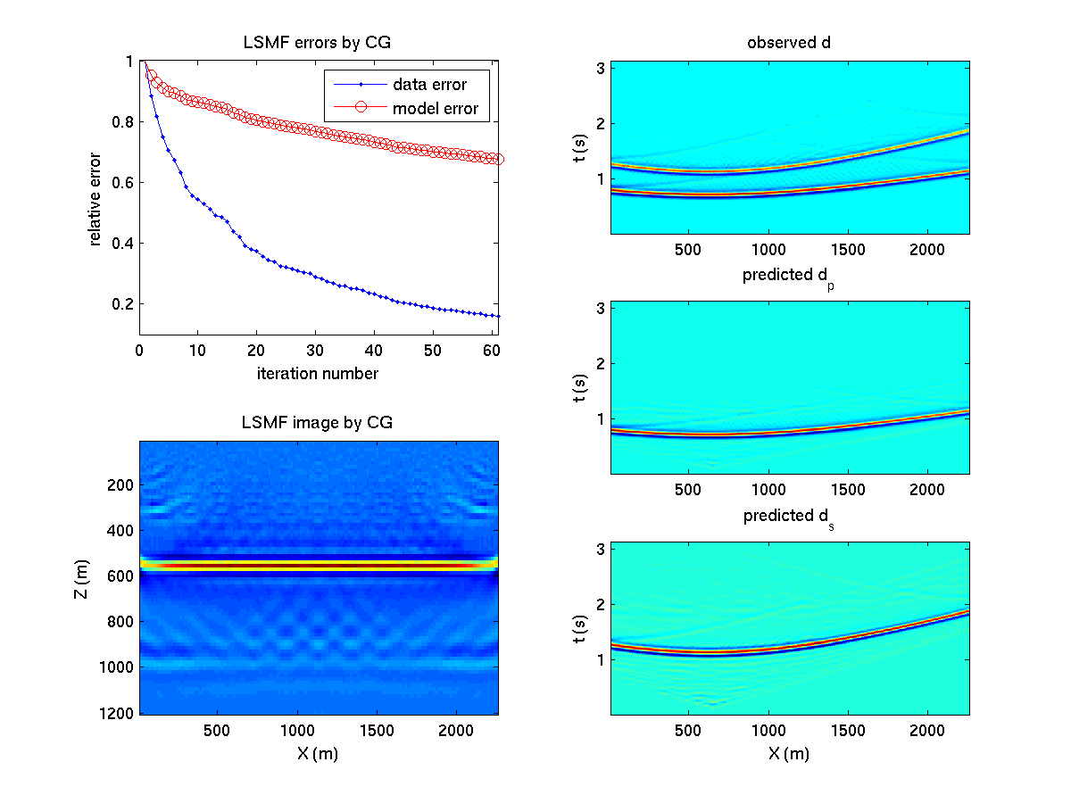
The number of sources and receivers are 12 and 150, respectively. The right column of the panels shows the data separation results.
Objective: Learn how to carry out LSMF, using Born modeling and conjugate gradient (CG) method.
Procedure:
- Download the codes LSMF_m_files.tgz.
Run: tar -xzf LSMF_m_files.tgz
Then in you MATLAB command, cd to this newly created directory. - In MATLAB, run the script LSMF_script.m
Wait about 5 minutes (on a LINUX workstation with 12 cores) and Figure 1 will be generated.
The MATLAB files are well-commented. You may need to read the files to get an understanding. - Questions: in the lower left panel of Figure 1, besides one strong reflector at the correct depth, there are one weak and broken reflector at depth 320m and one weak reflector with many migration artifacts at depth 1000m.
Why do those two weak reflector arise? What migration operators and subsets of data are they associated with? - Investigate the sensitivity with respect to the velocities. Change the P- and S- velocities by 5%, and see how the results change.
Note that please do not change the velocities used to generate the observed data. Only change the velocities used in LSMF. You need to obtain new traveltime tables associated with the modified velocities, and then define the new L and Lt (i.e., forward and migration) operators to be used in LSMF.