2D Wave-Equation Interferometric Migration of VSP Multiples
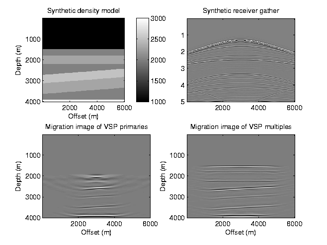
Figure 1. In this model, there are 600 shots evenly deployed on the surface, and 12 geophones evenly placed in the center well (offset 3000 m) at the depth range from 1900 m to 2120 m. From it we can see, migration of VSP multiples has a much larger imaging area than migration of VSP primaries.
Objective:
Learn to use 2D wave-equation interferometric migration (WEIM), and study its advantage in migration of VSP multiples.
Skill Learned:
A version of 2D WEIM implementation which can be extended for real data imaging.
Lesson learned
- Interferometric migration is robust to velocity estimation errors.
- Migration of VSP multiples has an imaging area comparable to that of a CDP survey.
Procedure:
- Make a directory, and load into it the file:
mmig.m,
- Download data: s.mat, d191.mat and mt1.mat into the same directory.
- Type "mmig;" in Matlab to run the program for migration of one geophone gather.
- Now, download other 11 geophone gathers:
d193.mat,
d195.mat,
d197.mat,
d199.mat,
d201.mat,
d203.mat,
d205.mat,
d207.mat,
d209.mat,
d211.mat,
d213.mat,
and traveltimes:
mt2.mat,
mt3.mat,
mt4.mat,
mt5.mat,
mt6.mat,
mt7.mat,
mt8.mat,
mt9.mat,
mt10.mat,
mt11.mat,
mt12.mat,
and density:
den.mat,
into the same directory.
- Change the corresponding file names in "mmig.m", and run the program for migration of each geophone gather.
- Stack all the migration images.
Questions to think about:
- What are the advantages of migrating VSP multiples? Why it is successful?
- What are the advantages of interferometric migration?
- Where are the artifacts from? And how to suppress them?
- How to determine the optimal geophone placement in the well?