Finite Difference Solution to the Acoustic Wave Equation
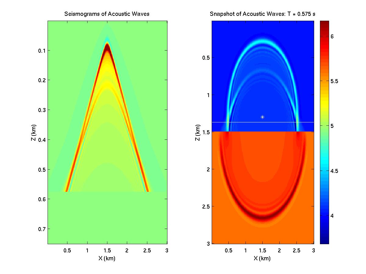
Figure 1. Seismograms and snapshot associated with a line source placed
just above the 2-layer medium.
Objective: Calculate synthetic seismograms by a 2-2 FD solution to the wave equation. Learn how space and time sampling increments affect the output.
Skill Learned: Implementation, design and construction of synthetic seismograms by finite-difference solutions to the wave equation.
Procedure:
- Download the codes fd.m and plt.m and type "fd". This will generate the synthetic seismograms and snapshots for a 2-layer medium.
Exercises:
- From the snapshots estimate the wavelengths of the waves in the top and bottom layers (Use the zoom facility in MATLAB). Compare these wavelengths to the theoretical estimates from lambda=c/f..
- Change ABCs so they are on all sides except for the top boundary..make the top a free surface. Repeat simulations. Describe the changes in snapshots compared to previous simulation.
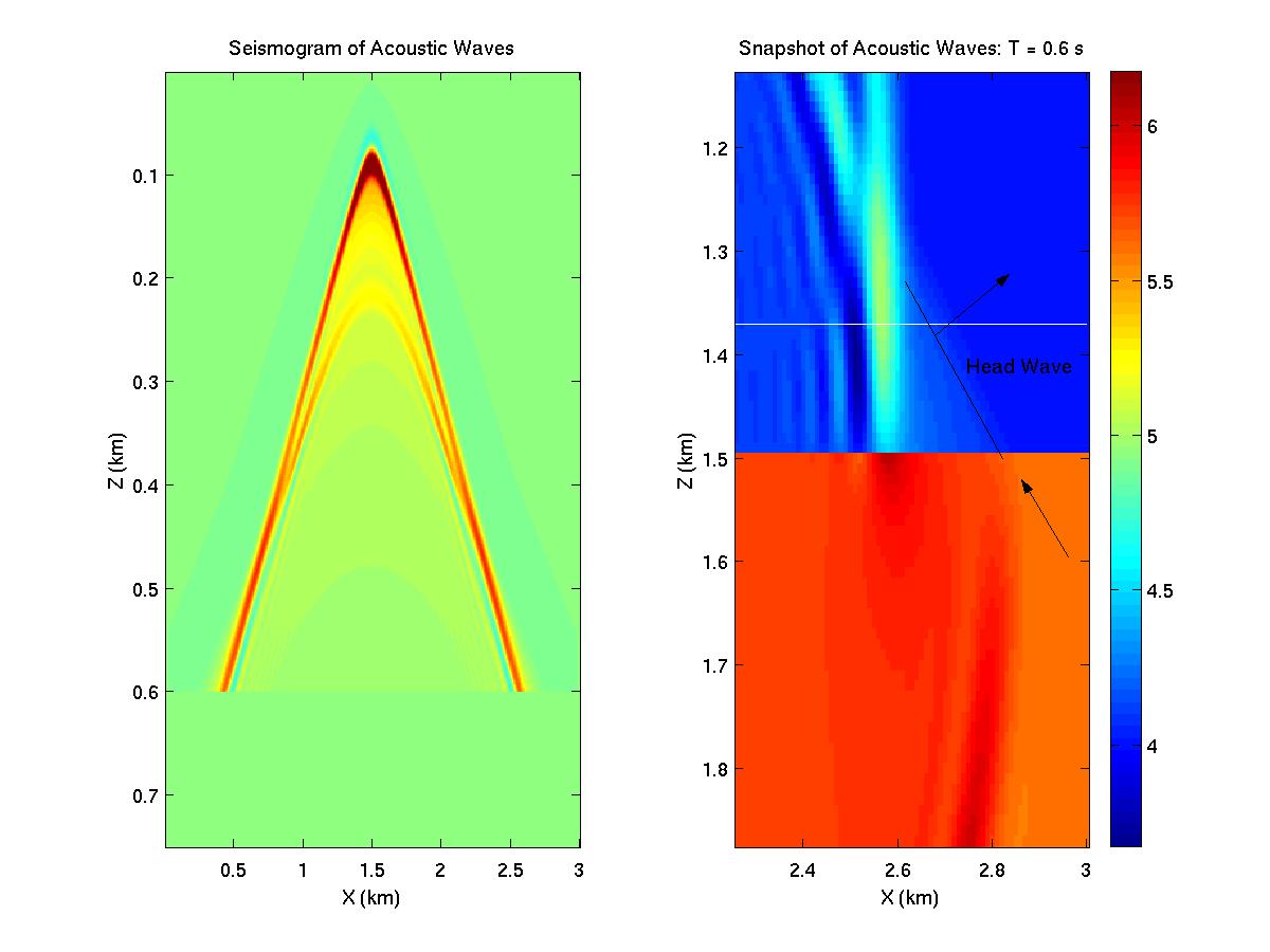
- Identify the direct, refraction, and reflection waves in the snapshots and the seismograms. Estimate their apparent velocities. Explain why the reflection waves moveout with the slowest apparent velocities.
- Raise the frequency of the source by 50% and repeat the simulations. Comment on loss of accuracy and give rationale.
- Choose a dt value that violates stability. Rerun simulations. What happens?
- The head wave arrival is extremely weak, as predicted by theory. However, a diving wave that gets trapped in a thin interface just below the refracting interface can boost up the amplitude. Adjust the velocity model so there is a thin layer (10 points thick) just below the original interface. make sure the velocity is the average between layer 1 and 2. Now rerun the fd.m code. Is there a difference in head wave amplitudes? Change models until you get a satisfactory amplitude.