Contents

CGAN LAB

Learn how to to do CGAN

================= Load Keras Modules and MNIST Dataset=================

#Import Keras Modules
%matplotlib inline
import matplotlib.pyplot as plt
import numpy as np

from keras.datasets import mnist
from keras.layers import (
        Activation, BatchNormalization, Concatenate, Dense,
        Embedding, Flatten, Input, Multiply, Reshape)
from keras.layers.advanced_activations import LeakyReLU
from keras.layers.convolutional import Conv2D, Conv2DTranspose
from keras.models import Model, Sequential
from keras.optimizers import Adam

================= Set up variables=================

img_rows and img_cols : Specify the input image size

channels : in this case the images are grayscale, so 1 channel

z_dim: Size of the noise vector z

please note in this case we are dealing with smaller images, 28x28. Commonly most tutorials use a z_dim of 100. However, 
if you have larger images, increasing your z_dim is benificial if your images are bigger. I have read making your z_dim a base of 2,
is easier on the GPUs, while others say a base 10.

num_classes : Number of classes/categories in our dataset

img_rows = 28
img_cols = 28
channels = 1
img_shape = (img_rows, img_cols, channels)
z_dim = 100
num_classes = 10

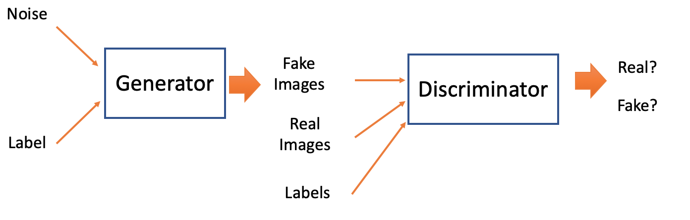
================= CGAN Generator=================

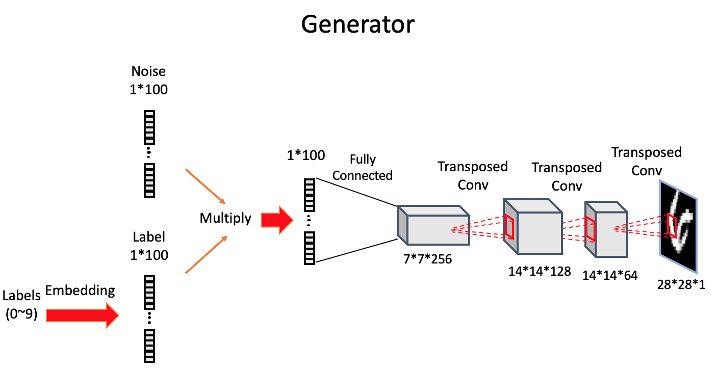
we use embedding and element-wise multiplication to combine the random noise vector z and the label y into a joint representation

1. Take label y (0-9), turn it into dense vector of size z_dim -(length of random noise vector) and use Keras Embedding layer.

2. Combine label embedding with noise vector z into joint representation with Keras Multiply layer -This layer multiplies corresponding entries of two equal-length vectors and outputs a single vector of resulting products

3. Feed resulting vector as input into CGAN Generator network to synthesize an image.

The resulting joined representation is used as input into CGAN Generator network

NOTE: please note, here you will make appropriate changes to your Dense layers and Reshape method according to the specifications of the dimensions of your own data. Here is where changes can be made to the generator to adapt to your specific CGAN use

Figure 2: Generator Structure

def build_generator(z_dim):

    model = Sequential()

    model.add(Dense(256 * 7 * 7, input_dim=z_dim))
    model.add(Reshape((7, 7, 256)))

    model.add(Conv2DTranspose(128, kernel_size=3, strides=2, padding='same'))

    model.add(BatchNormalization())

    model.add(LeakyReLU(alpha=0.01))

    model.add(Conv2DTranspose(64, kernel_size=3, strides=1, padding='same'))

    model.add(BatchNormalization())

    model.add(LeakyReLU(alpha=0.01))

    model.add(Conv2DTranspose(1, kernel_size=3, strides=2, padding='same'))

    model.add(Activation('tanh'))

    return model
def build_cgan_generator(z_dim):

    z = Input(shape=(z_dim, ))

    label = Input(shape=(1, ), dtype='int32')

    label_embedding = Embedding(num_classes, z_dim, input_length=1)(label)

    label_embedding = Flatten()(label_embedding)

    joined_representation = Multiply()([z, label_embedding])

    generator = build_generator(z_dim)

    conditioned_img = generator(joined_representation)

    return Model([z, label], conditioned_img)

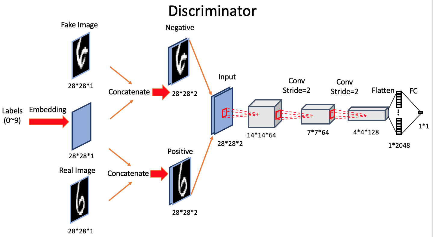
================ CGAN Discriminator ================

Here we handle the input image and its label

1. Take label (0-9), use Keras Embedding layer—turn label into dense vector of size (28×28×1=784) (length of flattened image).

2. Reshape label embeddings into image dimensions (28×28×1).

3. Concatenate reshaped label embedding onto corresponding image, creating joint representation with shape (28×28×2).

   • This is like an embedded label “stamped” on top of it.

4. Feed image-label joint representation as input into CGAN Discriminator network

   --Adjust the model input dimensions to (28×28×2) to reflect the new input shape.

At the output layer, we use a sigmoid activation function to produce a probability that the input image-label pair is real rather than fake—no change here.

Figure 3: Discriminator Structure

def build_discriminator(img_shape):

    model = Sequential()

    model.add(

        Conv2D(64,
               kernel_size=3,
               strides=2,
               input_shape=(img_shape[0], img_shape[1], img_shape[2] + 1),
               padding='same'))

    model.add(LeakyReLU(alpha=0.01))

    model.add(
        Conv2D(64,
               kernel_size=3,
               strides=2,
               input_shape=img_shape,
               padding='same'))

    model.add(BatchNormalization())

    model.add(LeakyReLU(alpha=0.01))

    model.add(
        Conv2D(128,
               kernel_size=3,
               strides=2,
               input_shape=img_shape,
               padding='same'))

    model.add(BatchNormalization())

    model.add(LeakyReLU(alpha=0.01))

    model.add(Flatten())
    model.add(Dense(1, activation='sigmoid'))

    return model


def build_cgan_discriminator(img_shape):

    img = Input(shape=img_shape)

    label = Input(shape=(1, ), dtype='int32')

    label_embedding = Embedding(num_classes,
                                np.prod(img_shape),
                                input_length=1)(label)

    label_embedding = Flatten()(label_embedding)

    label_embedding = Reshape(img_shape)(label_embedding)

    concatenated = Concatenate(axis=-1)([img, label_embedding])

    discriminator = build_discriminator(img_shape)

    classification = discriminator(concatenated)

    return Model([img, label], classification)

=================== Building the model ===================

build and compile the CGAN Discriminator and Generator models

the combined model used to train the Generator, the same input label is passed to the Generator (to generate a sample) and to the Discriminator (to make a prediction)

Figure 4: CGAN Structure

def build_cgan(generator, discriminator):

    z = Input(shape=(z_dim, ))

    label = Input(shape=(1, ))

    img = generator([z, label])

    classification = discriminator([img, label])

    model = Model([z, label], classification)

    return model


discriminator = build_cgan_discriminator(img_shape)
discriminator.compile(loss='binary_crossentropy',
                      optimizer=Adam(),
                      metrics=['accuracy'])

generator = build_cgan_generator(z_dim)

discriminator.trainable = False

cgan = build_cgan(generator, discriminator)
cgan.compile(loss='binary_crossentropy', optimizer=Adam())  

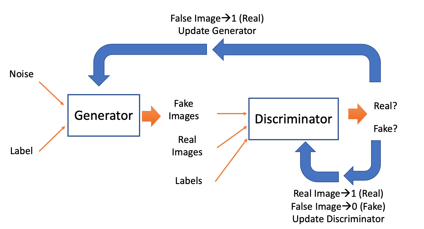
================= Function for Training =================

1. Take random mini-batch of real examples and their labels (x, y)

2. Compute D((x, y)) for mini-batch and backpropagate the binary classification loss to update θ(D) to minimize the loss

3. Take a mini-batch of random noise vectors and class labels (z, y) and generate a mini-batch of fake examples: G(z, y) = x*|y

4. Compute D(x*|y, y) for the mini-batch and backpropagate the binary classification loss to update θ(D) to minimize the loss.

5. Train the Generator:

   a) Take a mini-batch of random noise vectors and class labels (z, y) and generate a mini-batch of fake examples: G(z, y) = x*|y

   b) Compute D(x*|y, y) for given mini-batch and backpropagate binary classification loss to update θ(G) to maximize loss.

Figure 5: Training of CGAN Structure

accuracies = []
losses = []


def train(iterations, batch_size, sample_interval):

    (X_train, y_train), (_, _) = mnist.load_data()

    X_train = X_train / 127.5 - 1.
    X_train = np.expand_dims(X_train, axis=3)

    real = np.ones((batch_size, 1))

    fake = np.zeros((batch_size, 1))

    for iteration in range(iterations):



        idx = np.random.randint(0, X_train.shape[0], batch_size)
        imgs, labels = X_train[idx], y_train[idx]

        z = np.random.normal(0, 1, (batch_size, z_dim))
        gen_imgs = generator.predict([z, labels])

        d_loss_real = discriminator.train_on_batch([imgs, labels], real)
        d_loss_fake = discriminator.train_on_batch([gen_imgs, labels], fake)
        d_loss = 0.5 * np.add(d_loss_real, d_loss_fake)

        z = np.random.normal(0, 1, (batch_size, z_dim))

        labels = np.random.randint(0, num_classes, batch_size).reshape(-1, 1)

        g_loss = cgan.train_on_batch([z, labels], real)

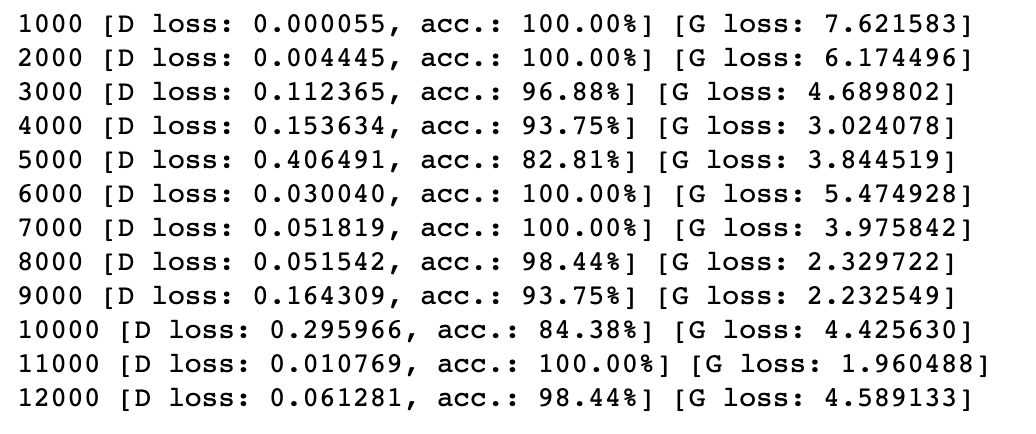
        if (iteration + 1) % sample_interval == 0:

            print("%d [D loss: %f, acc.: %.2f%%] [G loss: %f]" %
                  (iteration + 1, d_loss[0], 100 * d_loss[1], g_loss))

            losses.append((d_loss[0], g_loss))
            accuracies.append(100 * d_loss[1])

            sample_images()

================= Function for Outputting sample image=================

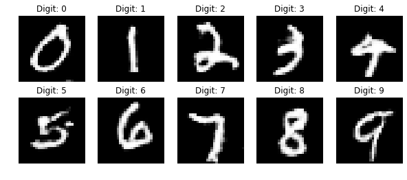
1. instead of a 4×4 grid of random handwritten digits, we generate a 2×5 grid of numbers: 1-5 in first row 6-9 in second row

   This allows inspection of how well the CGAN Generator is learning to produce specific numerals

2. we display the label for each example by using set_title() method

    def sample_images(image_grid_rows=2, image_grid_columns=5):

    z = np.random.normal(0, 1, (image_grid_rows * image_grid_columns, z_dim))

    labels = np.arange(0, 10).reshape(-1, 1)

    gen_imgs = generator.predict([z, labels])

    gen_imgs = 0.5 * gen_imgs + 0.5

    fig, axs = plt.subplots(image_grid_rows,
                            image_grid_columns,
                            figsize=(10, 4),
                            sharey=True,
                            sharex=True)

    cnt = 0
    for i in range(image_grid_rows):
        for j in range(image_grid_columns):
            axs[i, j].imshow(gen_imgs[cnt, :, :, 0], cmap='gray')
            axs[i, j].axis('off')
            axs[i, j].set_title("Digit: %d" % labels[cnt])
            cnt += 1
    

================= Function for Implement Model on Validation Set =================

# Plot predict results    
def plot_sample(X, y, preds, binary_preds, ix=None):

   """Function to plot the results"" 
   # ix is None, then random select image to plot
   if ix is None:
      ix = random.randint(0, len(X))
   fig, ax = plt.subplots(1, 4, figsize=(20, 10))
   # plot input seismic image
   ax[0].imshow(X[ix, ..., 0], cmap='seismic')
   # If there is salt in the image, plot the boundary of salt as black line
   has_mask = y[ix].max() > 0
   if has_mask:
      ax[0].contour(y[ix].squeeze(), colors='k', levels=[0.5])
   ax[0].set_title('Seismic')
   # plot true salt labels
   ax[1].imshow(y[ix].squeeze())
   ax[1].set_title('Salt')
   # Plot predicted salt probability 
   ax[2].imshow(preds[ix].squeeze(), vmin=0, vmax=1)
   if has_mask:
      ax[2].contour(y[ix].squeeze(), colors='k', levels=[0.5])
   ax[2].set_title('Salt Predicted')
   # Plot predicted salt Labels
   ax[3].imshow(binary_preds[ix].squeeze(), vmin=0, vmax=1)
   if has_mask:
      ax[3].contour(y[ix].squeeze(), colors='k', levels=[0.5])
   ax[3].set_title('Salt Predicted binary');
# Check if training data looks all right

plot_sample(X_train, y_train, preds_train, preds_train_t, ix=14) 
plot_sample(X_train, y_train, preds_train, preds_train_t)
# Check if validation data looks all right
plot_sample(X_valid, y_valid, preds_val, preds_val_t)

================= Training the Model=================

iterations = 12000
batch_size = 32
sample_interval = 1000

train(iterations, batch_size, sample_interval)

Figure 6: Output iteration numbers, loss functions and accuracy

Figure 7: Numbers generated by CGAN